Water Save
Project
Table of Contents
PROJECT DELIVERABLES
PROJECT OVERVIEW
SUMMARY
This is a data analysis project that contributes to the identification of the factors causing pipe failures and leakage in water supply systems and utilizes Python for the analysis.
PURPOSE & CONTEXT
This personal project is a product of my participation in CareerFoundry's Data Immersion Program. It provided me with an opportunity to delve into the analytical skills of Python, exploring the fundamentals of machine learning and modeling.
OBJECTIVE
The project objective is to increase the efficiency of the planning process for the rehabilitation of water supply systems as well as defining the risk of new pipe failures. The results of the analysis are expected to enable faster and more efficient identification of the factors causing pipe failures and leakage in water supply systems, and thus, to improve the current operational practice of the water utilities.
KEY QUESTIONS
- Explore the risk factors for the occurrence of pipe failures.
- Which risk factor is the dominant one?
- Which pipe material is the most apron to failure and under which conditions?
- Spatial distribution of the pipe failures.
- Is there any seasonably pattern in the occurrence of the pipe leakage?
- Forecast failures occurrence over time.
CREDITS
The research methodology has been developed as a part of the AWaRe project at the Karlsruhe Institute of Technology (KIT) and was funded by the German Federal Environmental Foundation DBU (Deutsche Bundesstiftung Umwelt).
Back to Table of ContentsTOOLS AND SKILLS


PROCESS
STEP 1: DATA Sourcing & Contents
Data Sourcing: The data was obtained by request from the municipal utility for the city of Pforzheim, Germany as a part of the research project AWaRe at the Karlsruhe Institute of Technology (KIT) and can be used only for academic or educational purposes.
Data Contents:
- dataset "pipelines" (originally named "leitungen.xlsx")
- dataset "failures" (originally named "schaeden.xlsx")
- dataset "Schadensdaten_geo"
The datasets contain information about the structural characteristics of the water pipelines, including specific characteristics like the material of the pipes, their diameter, age; and information about the environmental factors affecting the pipelines, like traffic loading, the level of groundwater, and the type of soil (considering soil aggressiveness and settlement) as well as details about the pipe failures that have occurred within the water supply network such as the date when the failure was reported, the cause for the pipe failure and the coordinates for reported failures.
Back to Table of ContentsSTEP 2: DATA WRANGLING & CONSISTENCY CHECKS
Data Wrangling: Involves tasks like dropping unnecessary columns, renaming columns for clarity, and adjusting variable data types. It ensures that the data is well-organized and suitable for analysis.
Data Consistency Checks: Identifying and rectifying mixed or incorrect data types, managing missing values, and addressing duplicates. Ensuring data quality and integrity is crucial for reliable analyses.
Back to Table of ContentsSTEP 3: GEOGRAPHICAL VISUALIZATIONS
During geographical visualizations with Python, utilizing libraries such as geopandas, folium, and pyproj allows creation of various types of maps. These include maps with clustered markers, heatmaps, and marker maps.
Visualizing Failures: Marker Map Illustrating the Spatial Distribution of the Pipe Failures and their Cause

Observation: The primary causes of failures result from soil movement and corrosion. However, both causes are equally distributed throughout the entire city area, making it challenging to pinpoint specific areas where the main cause can be identified. A detailed analysis is necessary to determine the factors contributing to the occurrence of failures in the water supply pipelines.
Heatmap: Visualizing the Spatial Density of Failure Points on the Map

Observation: The failures are concentrated in the center of the city, where the pipes are the oldest, indicating the initial growth phase of the network. To provide a clearer perspective on the influence of pipe age on failure occurrence, a visualization of pipes that experienced a failure, with annotations of the percentage relative to the total number of pipes for each age category, is presented. This visualization is part of the exploratory visual analysis, as described in the next step.
Visualization: Count and Percentage of Failures for each pipe Age Category
 Observation: The analysis indicates that the "old pipes" category (pipe age >= 50 years) has the highest percentage of failures among different pipe age categories. This observation logically suggests a recommendation for the rehabilitation planning of the water supply network. To prioritize and optimize replacement efforts, special attention should be given to the older pipes, particularly those exceeding 50 years.
However, it is crucial to conduct further analysis, considering the pipe material in relation to the number of failures. This additional examination will help understand whether older pipes with varying materials exhibit different patterns of failures. By identifying correlations between age, material, and failure occurrences, a more targeted and effective strategy for pipe replacement can be developed.
Back to Table of ContentsSTEP 4: EXPLORATORY VISUAL ANALYSIS
During exploratory analysis, relationships within the data are investigated. This includes employing tools like correlation matrices, heatmaps, scatterplots, as well as creating pair and categorical plots to gain insights into the underlying patterns and trends.
A. Key Question: Exploring pipe failures data categorized by pipe material, cause of occurrence and age category.
Tableau Snapshot: Overview of Pipe Failures Data (2002-2012)
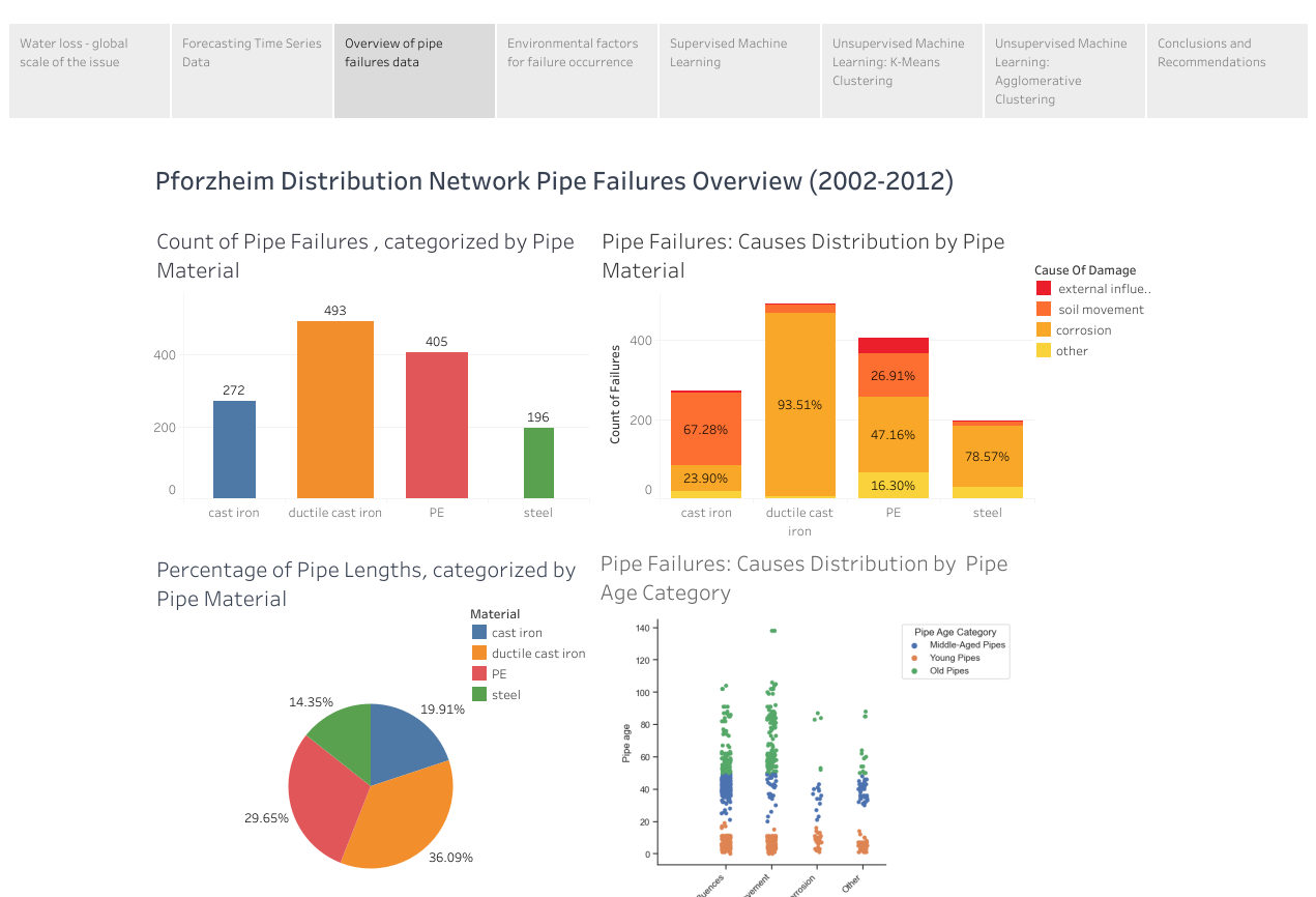
Visualization: Count of Pipe Material and Failure Cause Occurrences
 Note: Code for pipe material: 0 = unknown, 1 = asbestos cement, 2 = cast iron, 3 = ductile cast iron, 4 = steel , 5 = PE (polyethylene pipes), 8 = PE-100, 10 = PVC.
Code for cause of damage: 0 = unknown 1 = external influences, 2 = soil movement, 3 = corrosion, 4 = Deficiencies , 5 = Frost, 6 = Defective Socket, 7 = pipe connection, 8. bedding
Observation:
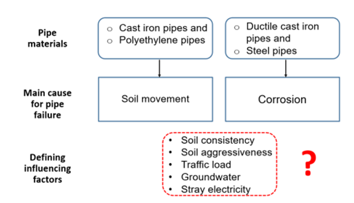
Cast Iron Pipes: Primarily found in the category of old pipes. The primary cause of failure is soil movement, with additional cases of corrosion and other factors.
Ductile Cast Iron Pipes: Predominantly present in the middle-aged and young pipes category. Corrosion stands out as the main cause of failure, though there are instances of failures due to soil movement and external influences.
Steel Pipes: Found in both old and middle-aged pipes categories. The main cause of failures is corrosion, with additional instances of failures attributed to soil movement, external influences, and other factors.
Polyethylene Pipes: Material PE is mainly observed in the middle-aged pipes category and material PE-100 in the young pipes. The data does not clearly indicate a dominant cause of failure. Failures are evenly distributed among soil movement, external influences, and other factors. Corrosion is not relevant for polyethylene pipes.
The analysis reveals two predominant causes of failure: soil movement and corrosion. Most failures in cast iron and polyethylene pipes are attributed to soil movement, while the primary cause of failures in ductile cast iron and steel pipes is corrosion. These findings underscore the necessity for a more in-depth examination, particularly in exploring external environmental factors that may contribute to failures. A comprehensive investigation is crucial to comprehend and define the impact of these external factors on the two main causes of failures: soil movement and corrosion. Additionally, ongoing analysis should address potential biases in the data, particularly concerning corrosion in polyethylene pipes.
B. Key Question: Exploring key environmental factors for the primary causes of failures.
Sample Visualizations:
Exploring soil aggressivity influence with correlation matrix and heatmap of occurrence frequency for combination of pipe material and soil aggressivity in 'cause of damage' categories 2 (soil movement) & 3 (corrosion)
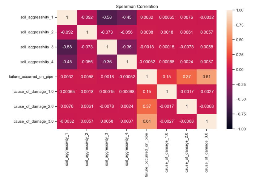
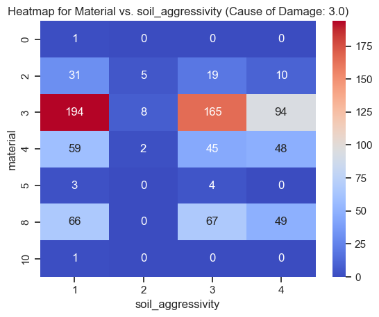
Analogous analyses were conducted for other environmental factors, including soil consistency, groundwater, traffic load, and stray electricity. Correlation matrices and heatmaps were generated to explore the frequency of occurrences for various combinations of pipe material and each environmental factor, providing a comprehensive understanding of their potential influences on the cause of damage categories.
Observation: Lack of strong correlation with failure occurrence. Upon reviewing the correlation matrix, no substantial correlation was observed between the analyzed factors, encompassing both structural and environmental elements, and the incidence of pipe failures. This indicates that the linear relationship between these specific factors and the occurrence of failures may not be statistically significant.
Interpretation: The absence of a strong correlation with failure occurrence suggests that the occurrence of failures is likely influenced by a combination of factors rather than individual factors in isolation.
Recommendation: Considering the limitations of the current analysis in comprehensively capturing the intricate relationship between environmental factors and the causes of pipe failure, particularly regarding specific pipe materials, it is recommended to incorporate machine learning models to gain a more thorough understanding of the factors influencing pipe failures.
Back to Table of ContentsSTEP 5: SUPERVISED MACHINE LEARNING
Building upon the preceding explanatory analysis, the following research hypotheses for examination through machine learning prediction models have been formulated: Critical environmental factors influencing the primary causes of failures in water supply pipelines encompass soil consistency, soil aggressivity, traffic load, and stray electricity. Additionally, it is proposed that the simultaneous presence of unfavorable soil consistency and excessive traffic loading contributes to failures in cast iron pipes. Moreover, it is suggested that the coexistence of unfavorable soil aggressivity and an unfavorable position of stray electricity is associated with failures in ductile cast iron and steel pipes.
In relation to the hypotheses, three models have been analyzed:
- Model 1 considers all critical environmental factors and includes all pipelines.
- Model 2 focuses on two environmental factors, soil consistency and traffic loading, which are crucial for cast iron pipes. Accordingly, the dataset has been limited to only cast iron pipes.
- Model 3 concentrates on the following two environmental factors: soil aggressivity and stray electricity, known to be critical for ductile cast iron and steel pipes. Consequently, the dataset has been restricted to including only those pipes.
At the outset, binary logistic regression was chosen for the analysis, given that the dependent variable, 'failure_occurred_on_pipe,' is characterized by binary values (0 – no occurrence of pipe failure or 1 – occurrence of pipe failure). Simultaneously, the independent variables exhibit a categorical nature. Logistic regression proves highly effective in scenarios where the outcome is binary.
Subsequently, the analysis results for Model 1 will be presented in the following section.
A. Binary Logistic Regression
1. Coefficients and odds ratios for the logistic regression model

- Codes for soil_consistency: 1= very low cohesive, 2= low cohesive, 3= moderately cohesive, 4= highly cohesive, 5= very highly cohesive.
- Codes for soil_aggressivity: 1= Ia (low), 2= Ib (low), 3= II (moderately), 4= III (highly).
- Codes for traffic_load: 1= none, 2= only passenger cars, 3= low (<100 trucks), 4= medium (up to 500 trucks), 5= high (up to 1000 trucks).
- Codes for stray_electricity: 1= 0 - 1 m distance to a pipeline, 2= 1 - 5 m distance to a pipeline, 3= 5 - 10 m, 4= more than 10 m distance to a pipeline.
The coefficients and odds ratios provide insights into how each variable is associated with the likelihood of the event (in this case, 'failure_occurred_on_pipe' being 1). These interpretations assume that the reference levels are very low cohesive soil consistency, no traffic, Ia (low) soil aggressivity, and stray electricity in the range of 0 - 1 m. An odds ratio greater than 1 indicates an increase in the odds of failure, while an odds ratio less than 1 indicates a decrease.
Observation:
a. Coefficients
- Soil Consistency: The coefficients indicate that soil consistency categories 2 and 5 contribute positively to the odds of failure, while categories 3 and 4 show negative impacts.
- Traffic Load: Higher traffic loads (categories 2, 3, 4, and 5) are associated with decreased odds of failure, with category 4 having the most significant impact.
- Soil Aggressivity: Category 4 exhibits a substantial positive impact on failure odds, while category 3 has a negative effect.
- Stray Electricity: Categories 3 and 4 show positive impacts on failure odds, while category 2 has a negative effect.
b. Odds Ratios
- Soil Consistency: Categories 2 and 5 increase the odds of failure by approximately 16.2% and 10.9%, respectively, while categories 3 and 4 decrease the odds by approximately 14.3% and 11.9%.
- Traffic Load: Higher traffic loads substantially decrease the odds of failure, with category 4 leading to a 48.8% reduction.
- Soil Aggressivity: Category 4 significantly increases the odds of failure by approximately 102.8%.
- Stray Electricity: Categories 3 and 4 increase the odds by approximately 56.6% and 15.7%, respectively.
Interpretation: While conventional expectations might suggest that unfavorable soil consistency, like highly to very highly cohesive soil, would exert the most significant impact on failure occurrence, the findings reveal mixed results where low or very highly cohesive soil demonstrates the most substantial influence. This pattern is consistent across other environmental factors as well. The variability in these results could stem from several factors, including multicollinearity, interactions between variables, and other unaccounted influences.
2. p-values and confidence intervals for the coefficients
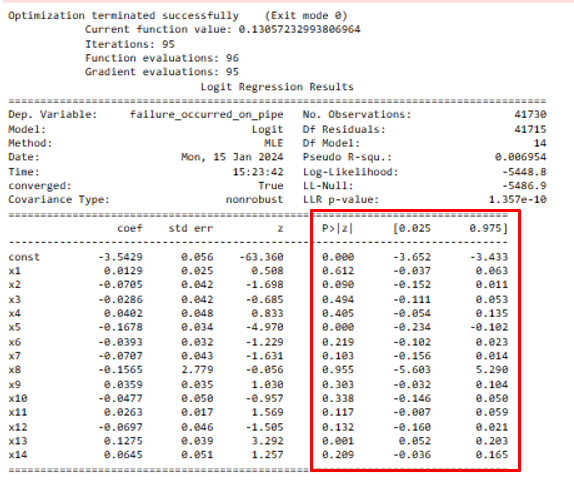
Observation: Upon examining the results for p-values and confidence intervals for the coefficients, it is evident that most of the variables (all except 'x5' and 'x13') have p-values greater than 0.05. This suggests that these variables may not be statistically significant predictors of the dependent variable. Only 'traffic_load_2' and 'stray_electricity_3' exhibit statistically significant associations, as indicated by their p-values below the 0.05 threshold.
Conclusion: It is crucial to note that while statistical significance provides valuable insights, it does not necessarily translate to practical significance. Considering the context of the study it appears illogical that only 'traffic_load_2' (limited to passenger cars) and 'stray_electricity_3' (in the range of 5 to 10 meters from the pipeline) exhibit statistical significance. This outcome may prompt further scrutiny into the model and variable selection, emphasizing the importance of practical relevance and the potential presence of intricate relationships among variables. Moreover, additional diagnostics, such as checking for multicollinearity, may be necessary to ensure the overall reliability of the results.
Checking for Multicollinearity Among Features by Calculating Variance Inflation Factor (VIF) for Each Independent Variable
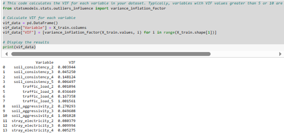
Observation: The calculated Variance Inflation Factor (VIF) values for each independent variable are remarkably low, indicating a minimal presence of multicollinearity among the predictors. Generally, VIF values below 5 or 10 are considered low, signifying that the precision of the estimated coefficients is not substantially influenced by multicollinearity.
3. Model Evaluation
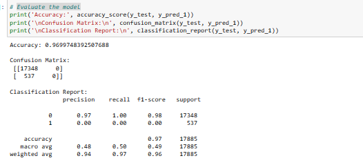
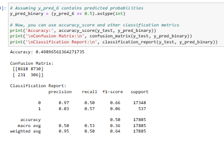
Observation:
The results show a high accuracy of 96.99%, but the confusion matrix and classification report reveal potential issues with the model's ability to predict the positive class (1).
- Precision: Precision for class 1 is 0, indicating that, of the instances predicted as positive, none were true positives.
- Recall (Sensitivity): Recall for class 1 is 0, suggesting that the model missed all instances of the positive class.
- F1-score: The F1-score for class 1 is 0, reflecting the poor performance in predicting the positive class.
- Support: The number of actual occurrences of each class in the specified dataset. The overall macro and weighted averages also highlight the imbalance in the classes.
In summary, while the model demonstrates high accuracy, its performance in identifying instances of the positive class is suboptimal due to dataset imbalance. To address this issue, I have incorporated techniques such as SMOTE (Synthetic Minority Over-Sampling Technique).
4. Imbalanced class handling, using SMOTE (Synthetic Minority Over-Sampling Technique)
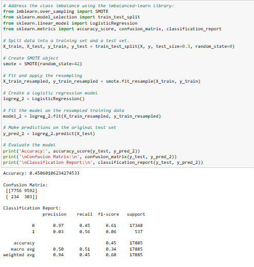
Observation: The accuracy has dropped significantly from 96.99% to 45.06% after applying SMOTE. The precision, recall, and f1-score for class 1 have slightly improved compared to the initial model, but they are still very low.
Conclusion: Even with the implementation of the SMOTE technique to address class imbalance, the model's effectiveness in capturing patterns within the minority class (1) remains limited. While accurate classifications for all instances of the negative class (0) have been achieved, further adjustments may be needed to enhance its predictive capabilities, particularly for the minority class.
Recommendation: Experimenting with different classification algorithms is advised. Some models, such as Random Forests or XGBoost Algorithm, might handle imbalanced datasets more effectively, potentially improving the model's performance in such scenarios.
B. Random Forests Algorithm
1. Model Evaluation
Observation: The model shows a comparable performance to the balanced Logistic Regression Model previously discussed. Despite efforts, the overall effectiveness of the model appears constrained, indicating that additional refinements might be necessary to improve its predictive capabilities.
2. Model’s feature importance scores
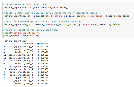
Observation: The scores are normalized and sum up to 1.0, indicating the proportion of importance that each feature contributes to the model. Features with higher importance scores are considered more influential in predicting the target variable, and consequently, features with lower scores are relatively less important in the model's predictions. In this instance, 'soil_aggressivity_3,' 'traffic_load_3,' and 'traffic_load_2' emerge as the most influential features. The identified influential features, such as 'soil_aggressivity_3' (moderately aggressive soil), 'traffic_load_3' (<100 trucks), and 'traffic_load_2' (only passenger cars), may lack clear, direct interpretations in the context of pipe failure.
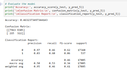
C. XGBoost Algorithm
1. Model Evaluation
Observation:
Conclusion: The models, regardless of the algorithm used, Logistic Regression, Random Forest or XGBoost Algorithm, are not performing well in predicting pipe failures based on environmental factors. There might be underlying challenges in capturing the patterns or relationships between environmental factors and pipe failures using the given features. To gain a deeper understanding, further exploration using advanced interpretability techniques or alternative modeling approaches is recommended.
Note: The results for Model 2 and Model 3 can be found on my GitHub profile. They yield similar outcomes, leading to the same pattern of conclusions as observed in Model 1.
Back to Table of ContentsSTEP 6: UNSUPERVISED MACHINE LEARNING, CLUSTER ANALYSIS IN PYTHON
In this step, the analysis of influencing factors, both structural and environmental, contributing to failure occurrence has been conducted by applying both K-Means clustering and Agglomerative Clustering techniques.
A. K-Means Clustering
Sample Visualizations:
1. Analyzing patterns in clusters data for the 'pipe diameter' and 'pipe age' variables
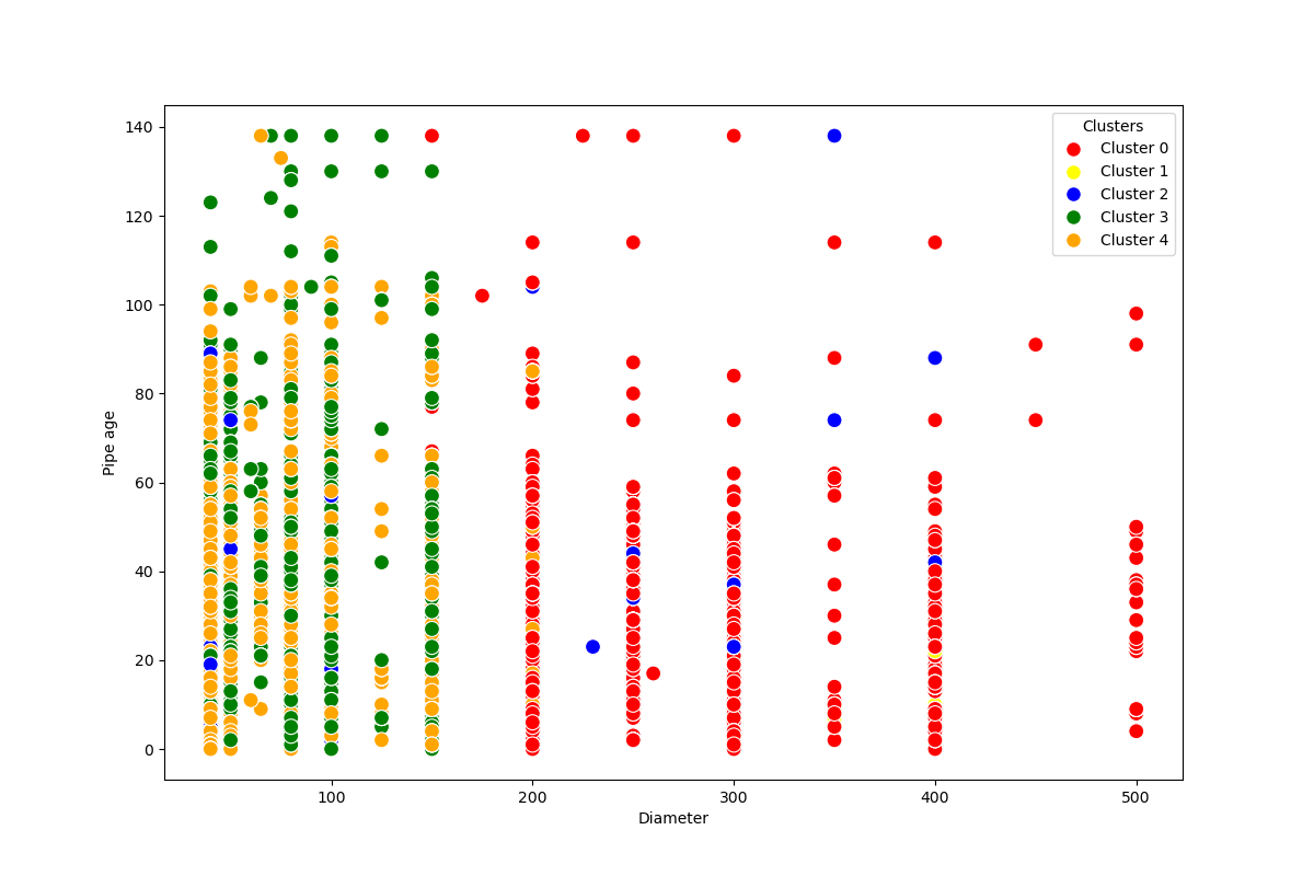
Observation: The visualization effectively reveals the distribution of pipe age and diameter across clusters. Clusters 3 and 4 primarily comprise smaller diameters, younger pipes, and middle-aged pipes. Cluster 0 is associated with medium to larger diameters, including both young and middle-aged pipes. Cluster 2 is characterized by older pipes, mostly with smaller to medium diameters. From this analysis of the clusters, we observe that there aren't any discernible patterns, except that the visualizations are logically presented and showcase that the entire range of pipe diameters present over the years.
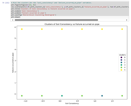
2. Analyzing patterns in standardized data clusters for the 'soil consistency' and the binary variable 'failure_occurred_on_pipe'
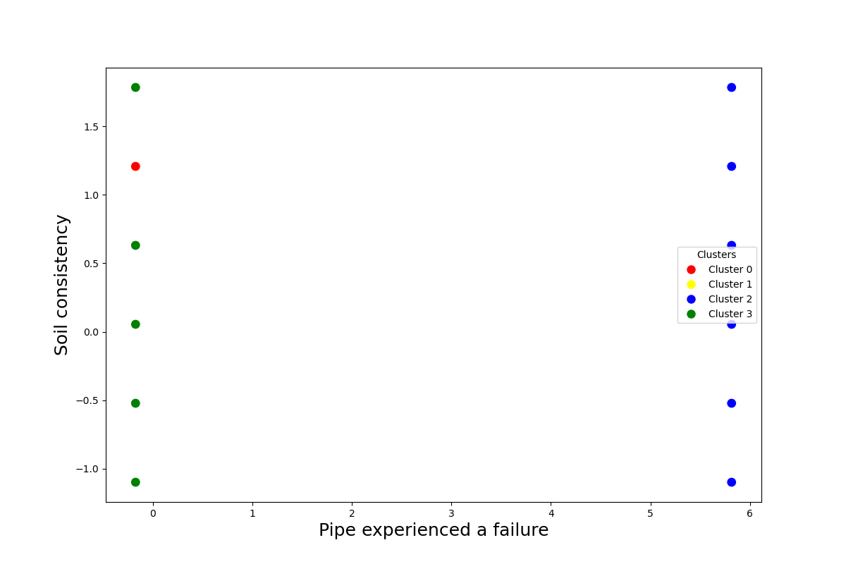
Observation:
Conclusion: Given the nature of the data, traditional clustering may not align with project goals, in the meaning of identifying influencing environmental factors.
Note: Sample visualizations are presented above, additional ones capturing other structural parameters, such as pipe length-diameter or pipe age-pipe length, as well as the influence factors with the binary variable 'failure_occurred_on_pipe,' are available on my GitHub profile.
B. Agglomerative Clustering
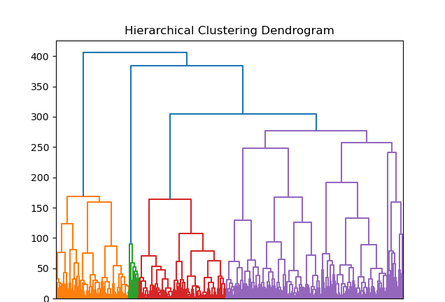
Sample Visualizations of the Clusters
Observation: Given the nature of the data, traditional clustering may not align with project goals, in the meaning of identifying influencing environmental factors.
Note: The rest of the Agglomerative Clustering visualizations are available on my GitHub profile.
Back to Table of ContentsSTEP 7: ANALYZING AND FORECASTING TIME SERIES DATA
This step entails the analysis and forecasting of the time series data depicting the distribution of failures over time.
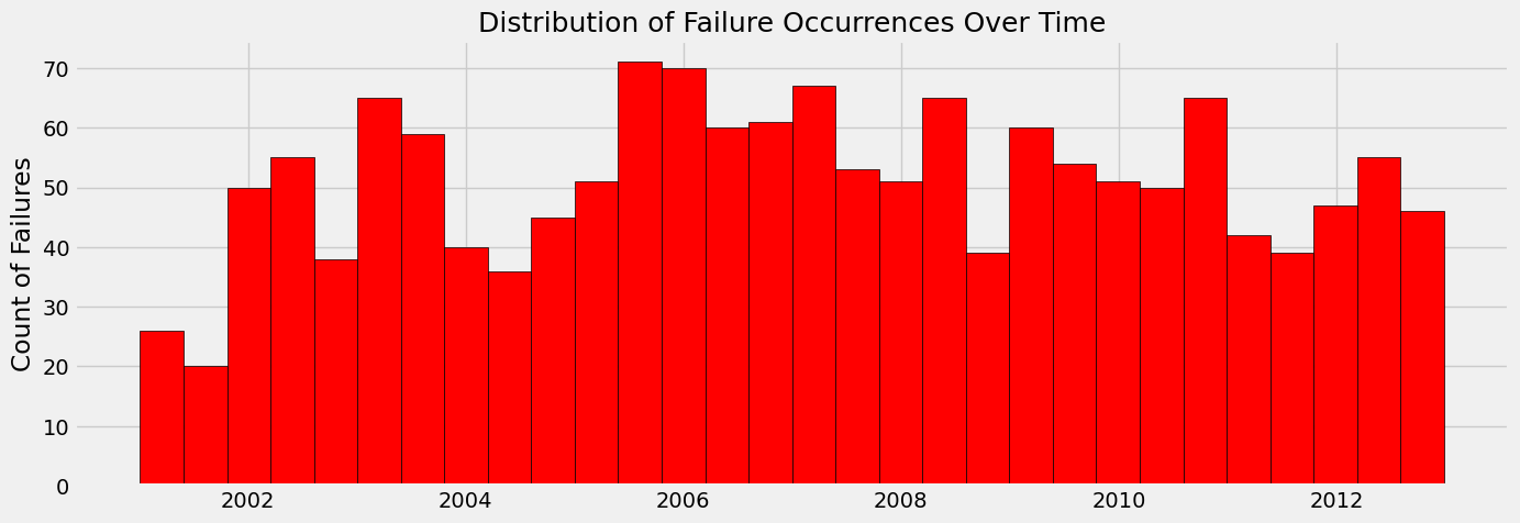
C. Key Question: Forecast Failures Occurrence Over Time
I. Analyzing phase
The analyzing phase involves decomposing the time series, testing for stationarity with Dickey-Fuller test, and checking for autocorrelation.
1. Decomposition of the data components
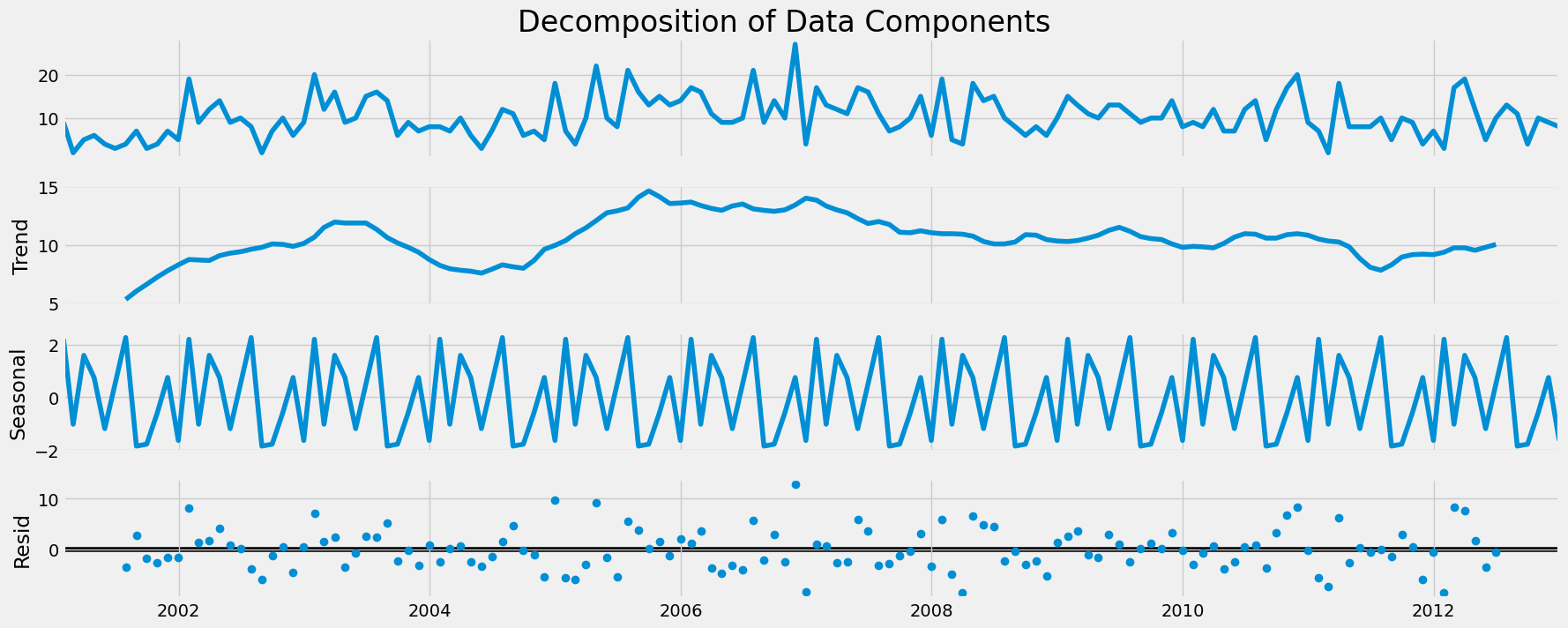
Observation:
- The first chart in the figure above is the data itself (including all its components).
- The second is the underlying trend. The level and trend of the data differ because there has been noise in the data. Noise represents any fluctuations that aren’t explained by the trend, so when the noise is removed (especially if there is a lot of it), the trend will likely differ. I don’t observe any trend in the data, which means the data are stationary, but anyhow I will perform stationarity test to make sure.
- The third component is seasonality. Here, I see seasonal fluctuations represented by a spikey curve that changes at a regular interval. If I didn’t have any seasonality, the curve would be flat.
- The fourth component is the noise—or, as it’s called here, “residual.” That is what’s left of the data after the trend and seasonality have been extracted (hence the term residual).
2. Testing for stationarity with Dickey-Fuller test
In this step, the stationarity of the time series data was assessed using the Dickey-Fuller test, a statistical test that examines the presence of a unit root.
Note: Rejecting the Null Hypothesis implies no unit root, indicating stationary data and allowing for forecast analysis. Forecast analysis is only feasible with stationary time series data.
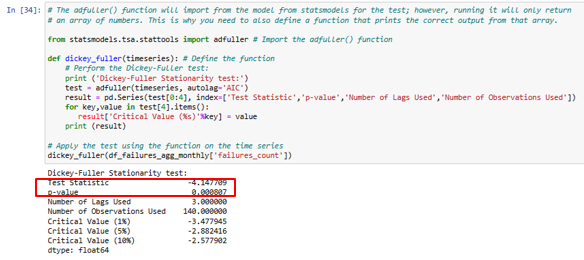
Observation: The test statistic (-4.15) is smaller than the critical value (-3.48), indicating that the null hypothesis can be rejected. This implies that the data is stationary. Additionally, the obtained p-value of 0.00081 (p < 0.05) further supports the rejection of the null hypothesis, confirming the stationarity of the data.
3. Checking for autocorrelation
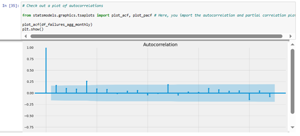
Observation: The vertical lines represent the lag values, indicating how many time periods in the past the correlation is calculated. The blue area (confidence interval) represents the confidence interval for the correlation values. If a vertical line crosses or goes beyond this area, it suggests that the correlation at that lag is statistically significant. In the above visualization, most of the lines (lag values) don't go beyond the confidence interval. This means there isn't a significant amount of autocorrelated data, and the dataset is likely stationary, supporting the result of the Dickey-Fuller test that has been conducted earlier.
II. Forecasting phase using ARMA (AutoRegressive Moving Average) Model
The forecasting phase encompasses tasks such as defining model parameters, data splitting, model running and fitting, and iterative refinement for enhanced accuracy.
Subsequently, I will present the final adjusted model obtained after iterative refinement for improved accuracy, while detailed steps of the forecasting phase can be found on my GitHub profile.
1. Summary of the ARMA model
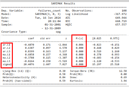
Observation: In the adjusted model, each coefficient (red box on the left) demonstrates statistical significance (p <= 0.05), red box on the right.
2. Visualization of the forecast model
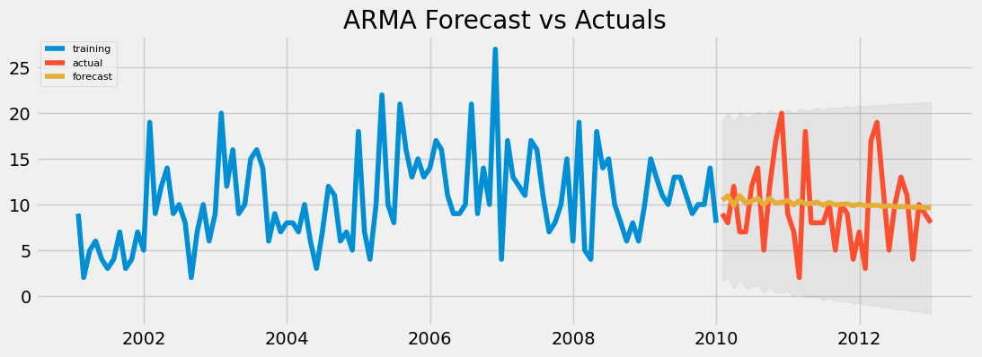
Observation: The projected forecast (indicated by the yellow line) does not precisely align with the observed actual values (depicted by the red line). Despite this, both trajectories fall within the confidence interval, indicating that they are not significantly distinguishable, reflecting a measure of success.
Back to Table of ContentsCONCLUSION AND RECOMMENDATIONS
ARMA Model Success
Accurately forecasting the occurrence of failures over time through effective utilization of the ARMA (AutoRegressive Moving Average) model.
Exploratory Analysis Insights
Most of the failures of the cast iron and polyethylene pipes occurred due to soil movement. Factors contributing to pipe failures induced by soil movement include unfavorable soil consistency, traffic loading, and groundwater influences.
The main cause of failures in ductile cast iron and steel pipes is corrosion. Corrosion-induced pipe failures are influenced by factors such as groundwater, soil aggressiveness, and the presence of power supply cables.
Machine Learning Challenges
Limited success in the identification of key influencing factors contributing to pipe failures using various Machine Learning Techniques.
Conclusion
The performance of models, such as Logistic Regression, Random Forest, and XGBoost Algorithm, appears suboptimal in identifying key influencing factors contributing to pipe failures. Furthermore, clustering methods have limitations in understanding these influencing factors. Given this, it is advisable to explore alternative approaches to enhance predictive accuracy.
Next steps
Given the data characteristics, Linear Extension of the Yule Process (LEYP) model is a promising choice. It incorporates multiplicative effects, accounting for past failures, aging, and covariates, which characterize the pipes and their environment, making it a more suitable option for further exploration.
Recommendation for Water Supply Network Rehabilitation Planning
To enhance the effectiveness and sustainability of water supply network rehabilitation, a comprehensive approach that addresses both material-specific causes of failure and age-based prioritization is essential. The following recommendations integrate insights from correlation analysis and emphasize targeted interventions tailored to the unique characteristics of pipe materials and aging infrastructure.
- Material-Specific Rehabilitation Approach:
- Age-Based Prioritization:
- Soil Movement Mitigation Measures:
- Corrosion Prevention Strategies:
- Data Quality Assurance and Bias Mitigation:
- Integration of Maintenance Protocols:
- Stakeholder Engagement and Public Awareness:
- Continuous Improvement and Adaptation:
Develop customized rehabilitation plans tailored to the predominant causes of failure identified for each pipe material.
Prioritize interventions targeting soil movement mitigation for cast iron and polyethylene pipes, while focusing on corrosion prevention measures for ductile cast iron and steel pipes.
Allocate resources to systematically assess and prioritize the replacement of aging infrastructure, with a focus on pipes exceeding the 50-year threshold.
Develop a comprehensive inventory detailing the age distribution of pipes to facilitate targeted rehabilitation efforts.
Implement engineering solutions such as soil stabilization techniques, trenchless technologies, and geotechnical assessments to mitigate the impact of soil movement on cast iron and polyethylene pipes.
Conduct regular inspections and monitoring to identify areas prone to soil movement and proactively address potential vulnerabilities.
Deploy corrosion-resistant coatings, cathodic protection systems, and corrosion inhibitors to safeguard ductile cast iron and steel pipes against corrosion-induced failures.
corrosion-related deterioration and implement timely interventions.
Continuously evaluate and refine the data collection methodologies to ensure accuracy, completeness, and representativeness of failure data, particularly concerning corrosion in polyethylene pipes.
Employ statistical techniques and sensitivity analyses to identify and mitigate potential biases, enhancing the reliability of correlation findings and informing evidence-based decision-making.
Integrate proactive maintenance protocols, such as regular inspections and condition assessments, to monitor the health of aging infrastructure and preemptively address potential vulnerabilities.
Implement a robust asset management system to track maintenance activities, facilitate data-driven decision-making, and ensure the long-term resilience of the water supply network.
Foster collaboration with relevant stakeholders, including local authorities, utility providers, and community members, to garner support for rehabilitation initiatives and promote awareness of the importance of infrastructure maintenance.
Communicate transparently with the public regarding rehabilitation plans, timelines, and anticipated impacts to cultivate understanding and cooperation.
Establish mechanisms for ongoing monitoring, evaluation, and refinement of the rehabilitation strategy based on evolving data insights, technological advancements, and changing infrastructure needs.
Embrace a culture of continuous improvement, innovation, and adaptability to ensure the effectiveness and sustainability of rehabilitation efforts over time.
By adopting a systematic and data-driven approach that integrates material-specific considerations and age-based prioritization, the water supply network can be rehabilitated in a targeted, efficient, and sustainable manner, safeguarding the reliability and resilience of essential water services for the community.
Back to Table of Contents- © Untitled
- Design: HTML5 UP